Structure of Data in the Google BigQuery Data Warehouse

Google BigQuery is a fully managed, highly scalable, cost-effective cloud data warehouse. It is a part of the Google Cloud Platform (GCP) suite of services. BigQuery uses Google’s framework to query and analyze large amounts of data quickly and efficiently. Further, as it is fully managed, BigQuery manages storage, provisions servers, and does resource sizing as necessary. Apart from this, with its partitioning and clustering features, you can control costs, improve query performance, and optimize data storage.

Google BigQuery Architecture

BigQuery is a completely managed service comprising four components shown in the following image:

• Compute Engine: All SQL queries in BigQuery are run by Dremel, its compute engine, which is a large multi-tenant cluster query engine. When you run a query, Dremel converts it into an execution tree, as shown in the diagram above:

  • The leaf nodes of the tree, called slots, read the data from the storage layer, process the query, and gather the results. Dremel dynamically allocates slots to queries from concurrent users. As a result, you can get thousands of slots to run your queries.

  • The branches, called mixers, aggregate the data.

  • The root node receives incoming queries from clients and routes the queries to the next level. It is responsible for returning query results to the client. BigQuery stores the data from the various stages of query execution in a layer called distributed memory shuffle until they are ready to be used.

• Distributed Storage: The data loaded to BigQuery is stored in Colossus, Google’s distributed file storage system. All data centers have their own Colossus clusters, making them fault-tolerant, available, and durable. The scalable architecture of Colossus allows BigQuery to process and analyze massive datasets. Colossus also maintains the metadata for any partitions and clusters you may have created using BigQuery’s partitioning and clustering feature.

• Cluster Manager: Google’s Borg system manages clusters and does job scheduling for BigQuery. It runs BigQuery jobs in a distributed and scalable manner and does resource allocation, workload management, and load balancing.

• Network: Google’s petabit (Pb) data center network, Jupiter, optimizes data transfer between the compute and storage layers of BigQuery. For each SQL query, its bandwidth of more than 6 Pb/s allows BigQuery to read and transfer terabytes of data in seconds.

BigQuery separates the storage and computing functions. This provides it the flexibility to scale them on-demand without user intervention.

---

Resource Model

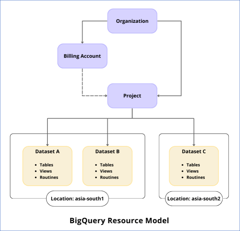
In BigQuery, resources are entities that you can use to manage and organize your data, resource permissions, quotas, slot reservations, and billing.

The entities in the BigQuery resource hierarchy include:

• Organization: The Organization resource is at the top of the Google Cloud resource hierarchy and represents a business or a company. All BigQuery resources are contained within this resource, thus enabling BigQuery administrators to control them centrally.

• Projects: Projects enable you to use all Google Cloud services. They are created in an organization resource. The tasks, called jobs, which run to perform actions on your BigQuery data, are created within a project.

• Datasets: Datasets are at the core of the BigQuery resource model. They are logical containers created in a GCP project for organizing the data. Each dataset has a location that you cannot change later. You can create several datasets in the same project based on your business needs. These datasets can be in diverse locations. Your BigQuery tables, views, functions, and procedures you add and their data are stored in the same location as the dataset.

  Your GCP project must be linked to an active Cloud Billing account if you want Hevo to load data into the datasets created in it. Any cost incurred by the project and its resources is billed to this account. Further, while configuring Google BigQuery as a Destination in Hevo, you can select an existing dataset, create one, or let Hevo create one for you.

The following image shows a sample resource hierarchy structure:

Data Structure

In BigQuery, data is stored in datasets. These are logical containers in which your BigQuery objects are created. Some of these objects are:

• Tables: Tables are the primary units of storage in a dataset. Data records are organized in rows, and each record is composed of columns or fields. Each BigQuery table is defined by a schema that describes the columns and their data types. You can create an empty table with or without a schema definition. In the latter case, you can provide the schema in the query that loads the data into your table. BigQuery uses this schema to define your table in the first run of the query.

• Views: Views are virtual tables that you can create by running SQL queries on the data in your BigQuery tables. You can use views for various reasons, such as, when you want to restrict the data visible to other users. You can also save a query as a view for easy access to relevant data. This query is run each time the view is accessed.

• User-defined Functions (UDFs) or Routines: Routines are a way to encapsulate reusable code and extend BigQuery’s SQL capabilities. These are stored procedures and functions that you can use to define custom logic and calculations on the data loaded to your tables.

---

Data Storage

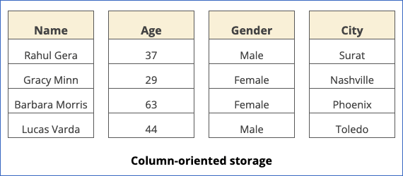
BigQuery uses a columnar format to store table data. This means that, unlike other SQL databases, each column of the data record or row is stored separately. Columnar storage optimizes query performance as it reduces the number of I/O requests made to fetch data. Being column-oriented allows BigQuery to scan and query data from large datasets efficiently.

In comparison to row-based storage, which is suited for transactional processing, column-based storage is optimal for analytical querying. Usually, an analytic query fetches data from a few columns in a table rather than the entire table. This makes BigQuery a good choice for a Destination when you need to aggregate a large amount of your Source data over several columns. Columnar data also enables greater data compression, as compression works better on similar data. This further improves the time that BigQuery takes to scan data.

The following example explains the two formats.

Example

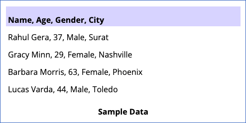
Consider the following set of data:

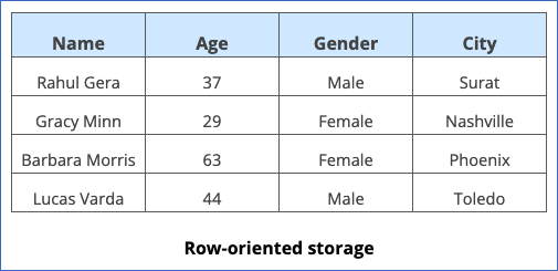
In a row-oriented format, the data would be written to the table one complete row at a time, as follows:

In a column-oriented format, such as in BigQuery, each row in the table would hold the data of one column, as follows:

Partitioning

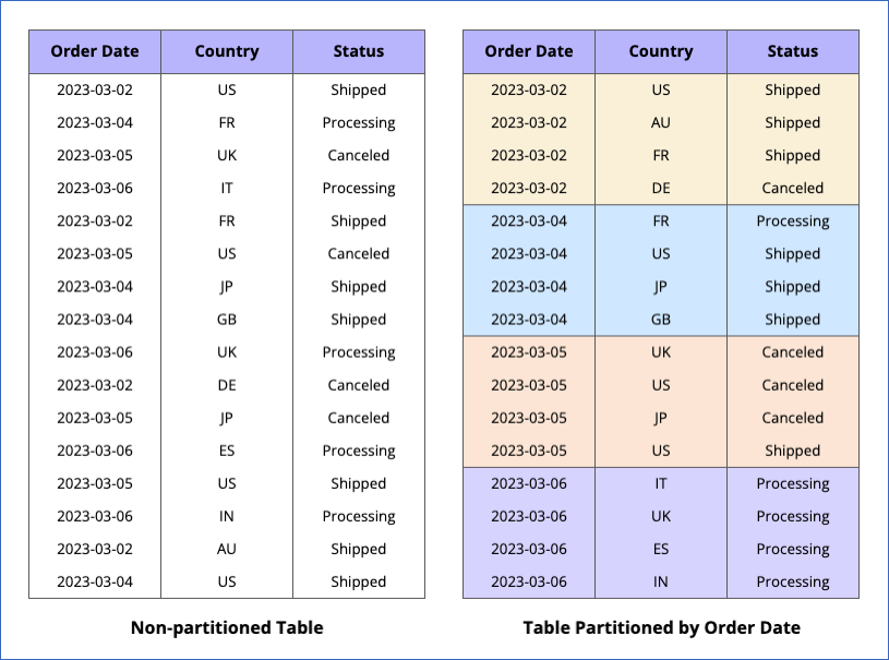
With the partitioning feature, you can divide large tables into smaller segments. These segments, called partitions, act as independent tables with one partition per table. Partitions are created based on the values in a partition key, and data is placed in them per the ingestion time, a time-unit column, or an integer range. You can use partitioned tables to improve query performance and control costs, as partitioning helps reduce the number of bytes scanned by the query.

The following image is an example of a table partitioned by Order Date. Suppose you query this table to fetch data where the Order Date is 2023-03-05. Now, in the case of a non-partitioned table, BigQuery scans the entire table and fetches the relevant records. However, when the data is partitioned by the Order Date, BigQuery does not scan the entire data. Instead, it only fetches data from the 2023-03-05 partition. This reduces your query cost while improving the time taken.

Read Partitioning in BigQuery and Recreating Partitioned Tables from BigQuery Console for information on creating partitioned tables.

Clustering

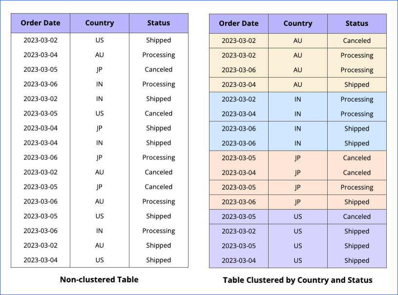
With the clustering feature, you can organize data based on the contents of the column(s) in a table. These columns, known as cluster keys, are used to collocate related data, and the order in which you specify them determines the sort order of data. In clustered tables, data is sorted into blocks based on common access patterns. BigQuery supports clustering for both partitioned and non-partitioned tables.

Clustering is particularly beneficial in scenarios when your data:

• Contains a large number of columns with distinct values, such as transactionId or orderId.

• Is frequently queried using the same columns together.

The following is an example of a table where data is clustered by Country and then by Status:

Read Clustering in BigQuery for information on creating clustered tables in Hevo.

BigQuery performs automatic re-clustering whenever new data is added to a clustered table or any partition in it. This is done to maintain the sort order of data in the table or partition.

Combining clustered and partitioned tables

You can combine clustering with partitioning to sort your data further and optimize query performance. This is because data is sorted into blocks as per the clustering columns in each partition. However, clustering works best with partitioning when:

• You work with large datasets with a clear pattern in data.

• Each partition can contain at least 1 GB of data.

• You want to estimate the query cost before it is run.

The following images are an example of how data is stored when a table is:

• Non-partitioned and non-clustered:

  

• Clustered by Country and Status:

  

• Partitioned by Order Date and clustered by Country:

  

Hevo uses BigQuery’s Batch Load feature to load the data it ingests from your Source into the BigQuery Destination tables. Using SQL queries, Hevo:

• Identifies the data to be copied to the target tables.

• If your Source data contains primary keys, it:

  • Copies the data to a temporary table.

  • Identifies and deletes duplicate data.

• Copies the data into the BigQuery tables.

Read Loading Data to a Google BigQuery Data Warehouse for details on the data loading process.

To improve the performance of the SQL queries that Hevo runs and lower their costs, you can create partitioned tables. Partitions make it easier to manage and query your data. Similarly, you can use clustered tables to narrow down the searches. Clustering allows you to organize and sort data by the patterns used to access it. You can use both these features to better the performance of the SQL queries that Hevo runs and reduce the amount of data that is scanned. Read When to use clustering to know when to use it over partitioning and vice versa.

---

Revision History